TEN PARTICLES - equilibrium thermodynamics
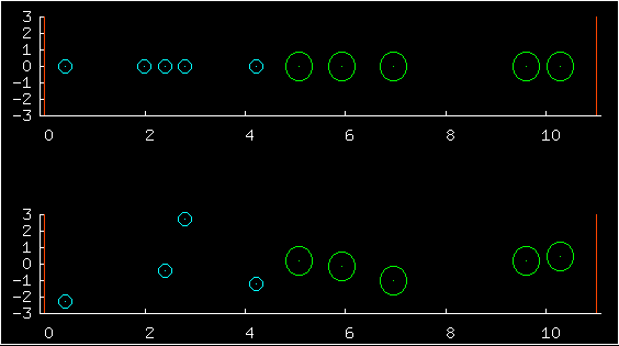 In the first multiplot, the upper half shows
the positions of ten particles, and the low half shows the complete
state - both the positions (horizontal coordinates) and the
velocities (vertical coordinates).
In the first multiplot, the upper half shows
the positions of ten particles, and the low half shows the complete
state - both the positions (horizontal coordinates) and the
velocities (vertical coordinates).
The blue particles on the left have masses roughly equal to 1.0. The green on the right have masses roughly equal to 4.0. One of the predictions of statistical physics is that for a large system at equilibrium, the probability of any state is just exp(-beta E)/Z, where E is the energy of the state. This prediction has astonishing consequences. First, each particle's velocity should have a Gaussian distribution. Second, all valid positions are equiprobable, and the probability of the positions and the velocities is a separable distribution -- positions and velocities are independent. All valid positions are equiprobable, whatever the masses of the particles are. So changing the particle masses may change their typical velocities but it has no effect at all on their typical positions.
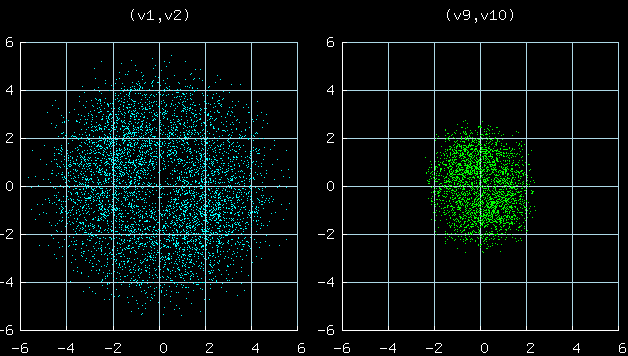 This figure shows scatter plots of the velocties of particles 1 and 2
(left) and particles 9 and 10 (right).
This figure shows scatter plots of the velocties of particles 1 and 2
(left) and particles 9 and 10 (right).
A striking prediction of statistical physics is that both
distributions should be Gaussian, and the standard deviations
of v1 and v10 (velocities of particles 1 and 10) should be
in the ratio 2:1, because the mass ratio is 1:4.
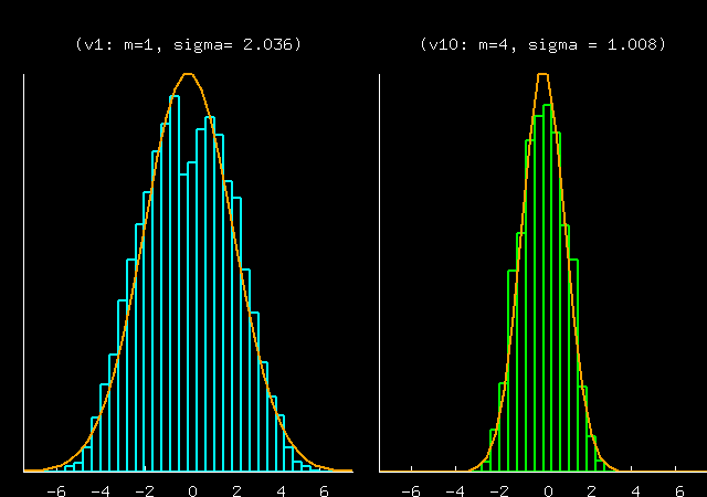 This prediction is well borne out in the data, though the
data show an intriguing dimple in P(v1) -- is this dimple because
N=10 is too small for the large-N equilibrium theory to
apply? Or is it because the particular random masses chosen here
give a system that has a slow mixing time, so the points
generated were not actually a good representation of the
equilibrium distribution?
This prediction is well borne out in the data, though the
data show an intriguing dimple in P(v1) -- is this dimple because
N=10 is too small for the large-N equilibrium theory to
apply? Or is it because the particular random masses chosen here
give a system that has a slow mixing time, so the points
generated were not actually a good representation of the
equilibrium distribution?
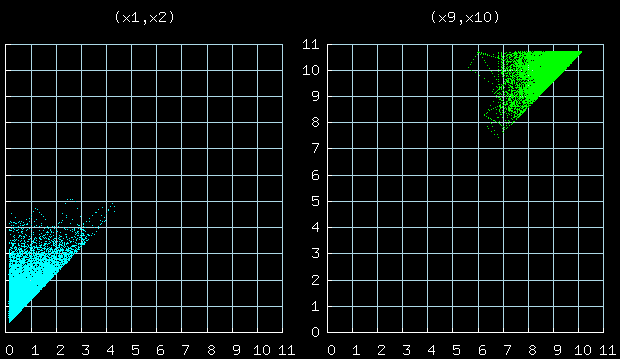 This figure shows the joint distribution of the positions of
particles 1 and 2, 9 and 10.
This figure shows the joint distribution of the positions of
particles 1 and 2, 9 and 10.
ELEVEN PARTICLES - non-equilibrium thermodynamics
The next pin-up in my picture gallery illustrates very different ideas. In the 10-particle example above,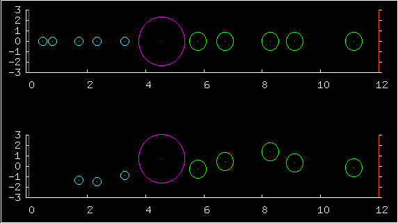 we were assuming that equilibrium had been reached
and testing the predictions of equilibrium theory.
In my eleven-particle example, I have a large purple particle
which I call the piston plopped in the middle. The dynamics
are the same as normal, but its mass (40) is so much bigger
than the others, the behaviour of them all is radically altered.
In this simulation I set off all the particles with equal velocities.
This means the situation is not at all typical of an equilibrium
thermal distribution -- the big guy has far too much energy -- he has
roughly 75% of the energy and at equilibrium he'd expect to have
9%. So what happens for the whole simulation is non-equilibrium.
One way of thinking of the piston is that he's a lot like a wall,
pushing down on the green community and rushing away from the
blue - or vice versa. What happens to a gas that is rapidly
compressed or expanded by a moving piston? Well, it
depends exactly which sort of expansion we are discussing, but
an adiabatic expansion is one sort.
If the blue community and the green community both behave like
adiabatically expanded or compressed gases, what
would you predict their temperature and pressure to do as
a function of 'volume' (which means the accessible volume
given the piston position)? Maybe the motion of the
piston can be modelled using the idea that its acceleration
is the result of the pressure difference between the green
gas on the right and the blue gas on the left?
Under this theory, the piston should move approximately like a
simple harmonic oscillator.
What frequency does the adiabatic theory predict?
we were assuming that equilibrium had been reached
and testing the predictions of equilibrium theory.
In my eleven-particle example, I have a large purple particle
which I call the piston plopped in the middle. The dynamics
are the same as normal, but its mass (40) is so much bigger
than the others, the behaviour of them all is radically altered.
In this simulation I set off all the particles with equal velocities.
This means the situation is not at all typical of an equilibrium
thermal distribution -- the big guy has far too much energy -- he has
roughly 75% of the energy and at equilibrium he'd expect to have
9%. So what happens for the whole simulation is non-equilibrium.
One way of thinking of the piston is that he's a lot like a wall,
pushing down on the green community and rushing away from the
blue - or vice versa. What happens to a gas that is rapidly
compressed or expanded by a moving piston? Well, it
depends exactly which sort of expansion we are discussing, but
an adiabatic expansion is one sort.
If the blue community and the green community both behave like
adiabatically expanded or compressed gases, what
would you predict their temperature and pressure to do as
a function of 'volume' (which means the accessible volume
given the piston position)? Maybe the motion of the
piston can be modelled using the idea that its acceleration
is the result of the pressure difference between the green
gas on the right and the blue gas on the left?
Under this theory, the piston should move approximately like a
simple harmonic oscillator.
What frequency does the adiabatic theory predict?
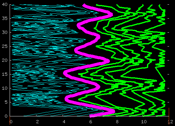 Here's the positions (horizontal axis) of all the particles
as a function of time (vertical axis).
Here's the positions (horizontal axis) of all the particles
as a function of time (vertical axis).
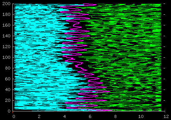 Here's the same thing but showing more data.
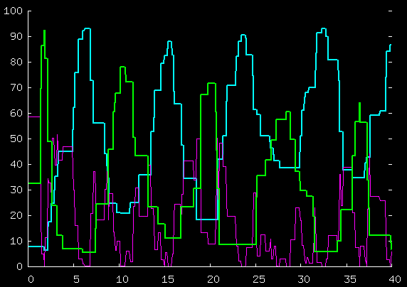 Here's the total kinetic energy of the blue guys,
the green guys, and the purple guy, for the first 40 time units;
Here's the total kinetic energy of the blue guys,
the green guys, and the purple guy, for the first 40 time units;
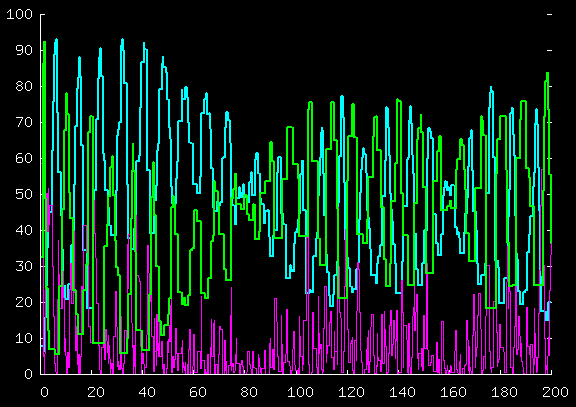 and for the first 200 time units.
The way in which the excess
energy of the piston is gradually dissipated
and the energy sloshes between the particles
deserves hours of study and thought. If the piston had
very large mass, how would it ever lose energy to the
gases? Perhaps this is
a good test-bed for thinking about concepts of
fluctuations and dissipations.
and for the first 200 time units.
The way in which the excess
energy of the piston is gradually dissipated
and the energy sloshes between the particles
deserves hours of study and thought. If the piston had
very large mass, how would it ever lose energy to the
gases? Perhaps this is
a good test-bed for thinking about concepts of
fluctuations and dissipations.