back to Computational
Physics home page
Computing project: PLANET - solution in Octave
Note
I recommend using the command
gset size ratio -1
to make the plot have
equal size units on both axes.
You can also use
axis('equal')
to get the same result.
Similarly, instead of gset size noratio
you can use
axis('normal').
|
Solutions |
|
planet0.m | simple solution that
plots inside the loop
(uses gplot)
| |
planet0a.m | simple solution that
plots inside the loop
(uses plot)
| |
planet0C.m |
plots inside the loop
(uses plot, and has a delay of 0.02 seconds between plots. Uses the
commands time and pause)
|
|
planet10.m | uses a function, optionally
plots inside the loop, and returns a history matrix
(uses gplot)
|
|
RUNplanet10.m | example of how to call the planet10 function
using a script file
|
Alternatively, here is a command that runs planet10 directly.
planet10( [93,0] , [0,1.1] , 0 , 1000 , 1 , 0.015 , 10.0 );
|
RUNplanet11.m
doplot10.m
| script that (a) asks the user to choose an initial condition;
(b) runs planet10 (without plotting during the loop); then (c) plots
some graphs using doplot10.m.
|
RUNplanet12.m and
RUNplanet13.m.
| scripts that run through a fixed sequence of
initial conditions and makes a joint plot of all the resulting trajectories.
|
|
On this webpage
I have provided two files that contain
partial solutions to the planet project.
The two files are almost identical. The only difference
is that one uses "plot" to do the plotting, and
the other uses "gplot".
These files (planet0.m and planet0a.m)
are partial solutions, because they handle only
one initial condition, they do not use functions,
and they do not plot all the functions of interest.
Try running each of these: you will find
that the one that uses gplot runs quite a lot faster.
I think it might be a good idea to learn to use
gplot. The syntax for gplot is different from plot,
which means extra learning; but the syntax for gplot
is almost identical to the syntax for another plotting
program called gnuplot, so this extra learning
would not be a waste of time.
|
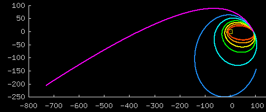 This graph shows 7 trajectories for initial
conditions, all of which start at the same point, and with
velocities in the same direction; the trajectories
differ by the magnitude of the initial velocity,
which goes from small (red) to large (blue and purple).
The initial velocity is directed along the tangent where
all 7 curves kiss each other.
In the first 6 cases, the resulting trajectory is bounded
(and is in fact an ellipse).
In the final purple case, the trajectory is unbounded (and is in fact a hyperbola).
The yellow box shows the sun.
This picture was made using
RUNplanet12.m.
This graph shows 7 trajectories for initial
conditions, all of which start at the same point, and with
velocities in the same direction; the trajectories
differ by the magnitude of the initial velocity,
which goes from small (red) to large (blue and purple).
The initial velocity is directed along the tangent where
all 7 curves kiss each other.
In the first 6 cases, the resulting trajectory is bounded
(and is in fact an ellipse).
In the final purple case, the trajectory is unbounded (and is in fact a hyperbola).
The yellow box shows the sun.
This picture was made using
RUNplanet12.m.
|
|
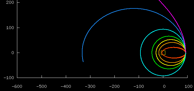 This graph shows 7 trajectories for initial
conditions, all of which start at the same point, and with
velocities in the same direction; the trajectories
differ by the magnitude of the initial velocity,
which goes from small (red) to large (blue and purple).
The initial velocity is directed exactly perpendicular to the line
joining the initial point to the sun.
In the first 6 cases, the resulting trajectory is bounded
(and is in fact an ellipse).
In the final purple case, the trajectory is unbounded (and is in fact a hyperbola).
Notice how most of the ellipses look a lot like circles.
This picture was made using
RUNplanet12.m.
This graph shows 7 trajectories for initial
conditions, all of which start at the same point, and with
velocities in the same direction; the trajectories
differ by the magnitude of the initial velocity,
which goes from small (red) to large (blue and purple).
The initial velocity is directed exactly perpendicular to the line
joining the initial point to the sun.
In the first 6 cases, the resulting trajectory is bounded
(and is in fact an ellipse).
In the final purple case, the trajectory is unbounded (and is in fact a hyperbola).
Notice how most of the ellipses look a lot like circles.
This picture was made using
RUNplanet12.m.
|
|
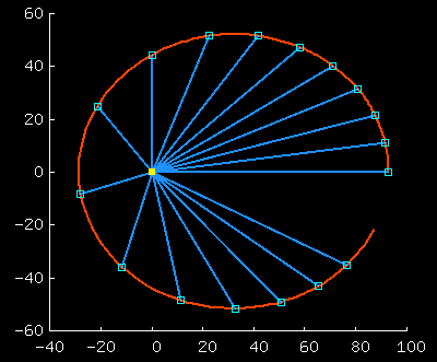
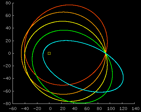 This graph shows 5 trajectories for initial
conditions, all of which start at the same point, with identical
speeds, but different directions.
(In all cases, the resulting trajectory is in fact an ellipse.)
This picture was made using
RUNplanet13.m.
This graph shows 5 trajectories for initial
conditions, all of which start at the same point, with identical
speeds, but different directions.
(In all cases, the resulting trajectory is in fact an ellipse.)
This picture was made using
RUNplanet13.m.
|