|
Here's a slightly fancier solution in which the particles have a
finite radius, to make better looking movies.
bounce2.m
is invoked by
cradle2.m
|
bounce2.m
more off
## Given a state (x,v) of length N and inverse-masses im(1..N)
## where x(1) = left-hand wall and im(1) = 0
## and x(N) = right hand wall and im(N) = 0
## determine which of the inter-particle collisions will take place next
## -- or is the next event one of the data-collection times {Tc, 2 Tc, 3Tc...}? --
## and simulate the motion until that event, and implement the collision.
time_to_next_clock = Tc ;
j = 0 ; ## counter: will run up to Number_samples_required
logbook = zeros(Number_samples_required , 2*N ) ;
########################################################################
## set up graph
figure(1);
y = zeros(size(x)) + ytweak ;
## look at the current velocities to guess a good range for the velocity graph
vmax=max(v);
vmin=max(-v) ;
vmax=max(vmax,vmin);
axis([x(1) (x(N)+xtweak(N)) -vmax*5.8 vmax*5.8]);
gset border 15
gset pointsize 8
gset nokey
########################################################################
## initialize lastplottime so that we think it is time to plot right away
lastplottime = time - time_between_plots ;
################################################################################
## Main loop:
## Keep simulating the motion until we have all the data we want
while ( j < Number_samples_required )
## run through all (left-hand) particles finding the time until collision with their
## right neighbours.
## Initialize the collisiontime vector to large positive numbers.
collisiontime=ones(1,N) * 2 * time_to_next_clock ;
## The Nth particle does not have a right neighbour, so we can use its "collision time"
## to store the time of the next clock event, which is when we will gather data for histograms
collisiontime(1,N) = time_to_next_clock ; ## this is used to indicate a clock event
for n=1:N-1
dv = v(1,n) - v(1,n+1) ;
## if the right neighbour is coming towards us (in our frame of reference)
## then work out when the collision would be
if ( dv > 0.0 )
collisiontime(n) = (x(1,n+1)-x(1,n))/dv ;
endif
endfor
## decide which collision needs to be rendered next
[a,b] = min( collisiontime ) ;
## simulate the motion for a time given by the min
dt = a ;
x = x + v * dt ;
time_to_next_clock = time_to_next_clock - dt ;
left = b ; ## b holds the index of the particle that has its collision next
if( left < N )
right = b+1;
## change the velocities of the dudes involved in a collision
[ v(1,left), v(1,right) ] = collide( v(1,left), v(1,right) , im(1,left), im(1,right) ) ;
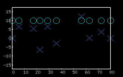
## plot( x , y , "x6" , x , v , "o3");
else
## no collision, it's clock time, so time to take a sample!
j ++ ;
if(doplot)
xyv = [ (x+xtweak)' ,y' ,v' ] ;
## elegant pausing rule that makes frame rate steady
timetillnextplot = lastplottime + time_between_plots - time ;
if ( timetillnextplot > 0.0 )
pause( timetillnextplot ) ;
timetillnextplot = 0.0 ;
else
## we are behind by the negative quantity timetillnextplot!
## to try to catch up, we will add this to "lastplottime" later
endif
gplot xyv u 1:2 w p 5 6, xyv u 1:3 w p 6 2
lastplottime = time + timetillnextplot ;
else
if( rem(j,1000) == 0 )
j
endif
endif
time_to_next_clock = Tc ;
logbook(j,:) = [x,v ] ;
endif
endwhile
|
|
bounce2.m
is invoked by
cradle2.m
|
cradle2.m
x = [ 0   14 15 16  17 18 19  20 21     35 ] ; N = 10 ;
## extra displacement to add to the particles so they appear to bounce
## off each other
xtweak = [ 0 : (N-1) ] * 5 ;
ytweak = 6;

## in cradle2 the masses are 4,9,1,1,1,1,1,1,1
## and the initial situation has all the energy in the left two masses
v = zeros(size(x) ) ;
im = zeros(size(x) ) ;
im(2:9) = 1.0 ;
im(2) = 1.0/4.123 ;
im(3) = 1.0/9.0123 ;

v(2:3) = - 2.0  ;

## this specifies how often in simulation time we make a plot
Tc = 0.2030123091;  Number_samples_required = 30000 ;  doplot = 1 ;
## this specifies how often in real time the plots will appear
time_between_plots = 0.025;

bounce2;
|
 that returns the new velocities of two particles
with inverse-masses im1 and im2,
after an elastic collision. (Momentum
is always conserved, in any collision between two isolated bodies.
An elastic collision
is one in which energy is conserved as well as momentum.)
The particles are moving in one dimension only.
The initial velocities
u1 and u2 can have any value, positive or negative or zero;
im1 and im2 can have any positive value, or zero (zero corresponds to the
inverse-mass of an enormous wall). [The inverse-masses are simply
im1 = 1/m1,
im2 = 1/m2.]
that returns the new velocities of two particles
with inverse-masses im1 and im2,
after an elastic collision. (Momentum
is always conserved, in any collision between two isolated bodies.
An elastic collision
is one in which energy is conserved as well as momentum.)
The particles are moving in one dimension only.
The initial velocities
u1 and u2 can have any value, positive or negative or zero;
im1 and im2 can have any positive value, or zero (zero corresponds to the
inverse-mass of an enormous wall). [The inverse-masses are simply
im1 = 1/m1,
im2 = 1/m2.]