|
In this example we plot a sin wave,
f(x) = sin(kx-wt)
and increase the value of t, replotting.
We then add up multiple sin waves, with different values of
wavenumber k
and frequency w, and plot the sum
for steadily increasing values of t.
|
The first example just plots one sinusoid.
Run it using
load 'gnu.wave'
from within gnuplot.
|
|
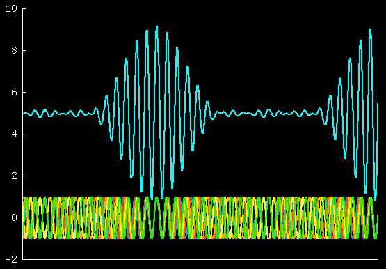
The next example plots two sinusoids and
their sum.
load 'gnu.wave2'
|
|
The next example shows how to make a movie
by using load 'gnu.wave4' to recursively carry out
functions that increment t and replot.
You should run this command -
load 'gnu.wave3'
|
|
- noting that that file loads this one, which
then loads itself again...
It loads itself forever, so you will need to hit Ctrl-C to stop it.
[Some window-managers have the annoying feature that
by default whenever a fresh plot happens in gnuplot, the window manager
gives focus to the gnuplot window; this default behaviour can be
disabled. I like to have focus follow the mouse.]
|
|
The next example rectifies the problem of the never-ending movie by
loading gnu.wave6 which contains an if
before its load command.
Run this example using
load 'gnu.wave5'
|
|
|
This file, gnu.wave6, is used by all the remaining examples.
|
|
|
You'll probably find that the previous example, gnu.wave5,
which increased the xrange of the plot,
produced a pretty lousy-looking plot, which didn't look like pictures
of sinusoids any more.
The problem was that the sinusoid has too many wiggles compared
with the default number of samples.
We fix this problem by cranking up the number of samples.
This file, gnu.wave7, shows how.
|
|
|
In these files, gnu.wave8 and gnu.wave9, we play around with the value of w2 a little,
seeing the effect of changing the dispersion relation.
|
|
|
This file, gnu.wave10, goes the whole hog, adding up
five sinusoids. Physicists may find it instructive to
play with the definition of the parameter dwdk.
|
|
|
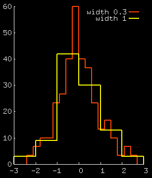
gnuplot has a function called fit
which can fit parameterized functions to data files
by twiddling whichever parameters you choose.
The objective function that is minimized by the fitting
process is the sum of squares of residuals.
[The residuals are the differences between the functions and
the data points.]
This is the standard objective function, widely used in data-fitting,
but do be careful to think whether it is an appropriate objective function.
It's appropriate, for example, if you wish to model the residuals
as coming independently and identically distributed from a gaussian
distribution.
fit is a pretty neat function. Its syntax is similar to
the plot syntax.
For this section, there are two data fails necessary to run the examples:
2006/Year and 2006/YearTd.
|
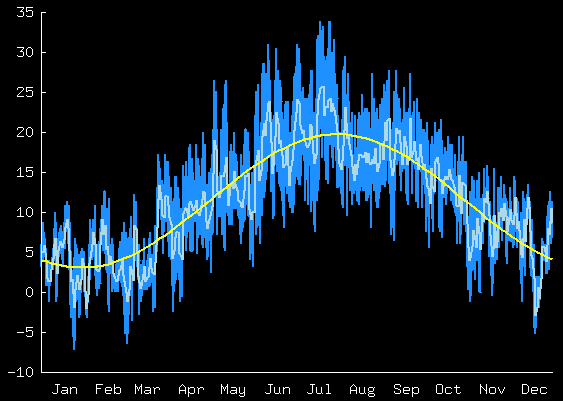
This first file, gnu.fit1, simply plots two data files,
one of which contains half-hourly temperature data, and one daily
averages of temperatures. It also plots a function
f(x) = A*sin( 2*pi* (x-o) / 365.0 ) + B,
a sinusoid with period 365 days,
whose parameters A, o, and B
are set to arbitrary values - i.e., the function hasn't been fitted.
The syntax of the plot command works like this:
plot '2006/Year' u ($0/48.0):($2) w l lt 6 ,\
 '2006/YearTd' u ($1-0.5):($2) w  l lt 8,\
 f(x)
-
First line - u ($0/48.0):($2)
means plot the line number ($0), divided by 48, on the x axis,
and plot column 2 ($2) on the y axis.
This line would work the same if it said
u ($0/48.0):2.
(There are 48 half-hours per day.)
- Second line - daily file - u ($1-0.5):($2)
means take the number in column 1
(which is the day number), subtract 0.5 from it,
and put that on the x-axis. Put the 2nd column on the y axis.
|
|
|
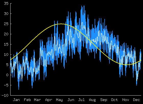
The second file, gnu.fit2, plots the data files and f(x)
as before, then runs the function
fit f(x) '2006/YearTd' u ($1-0.5):2 via A,o,B
so as to fit the function f(x) to the average daily data.
Note that the syntax of the "u" (using) part is the same
as used in the plot.
The words via A,o,B instruct the fit function
to vary those three parameters so as to optimize the fit of the function
f(x) to the specified data.
If all is well, this fit function will come up with a
good setting of the parameters, report them with error bars
and a correlation matrix, the stop;
the next command in the gnuplot file replots the function
so you can see how it fits.
|
|
|
|
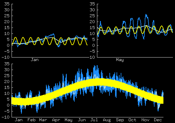
gnu.fit3 fits a more complicated model to the
half-hourly data - the temperature
is modelled as
the sum of two sinusoids, one with period one day, and one (as before) with
period one year.
Here the plot of the function is a fancy 'multiplot' with three
parts. To avoid writing everything twice, the details of the plot
command are popped into another file, gnu.showTempg, which
is loaded whenever we want to make the three-part plot.
|
|
|
|
|
|
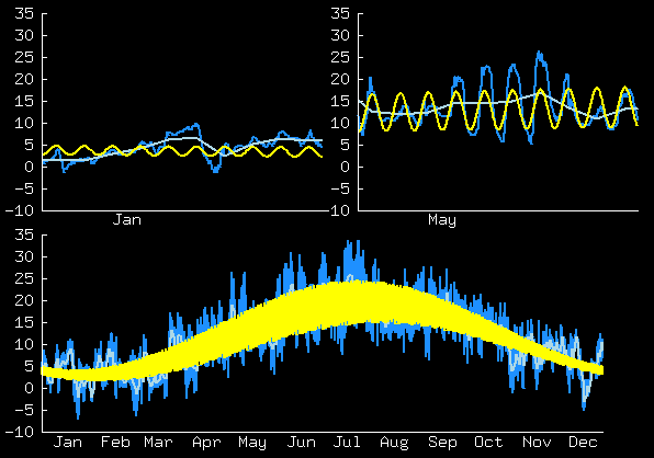
gnu.fit4 shows off fit's capabilities by fitting
a more complicated model, in which the daily sinusoid has an amplitude
that itself varies sinusoidally with a period of one year.
To find out more about fit, use ?fit
|
|
|
|
 This figure shows the circular orbit of the man,
his current velocity (magenta), and the velocity of the hammer
immediately post-kick (brown).
This figure shows the circular orbit of the man,
his current velocity (magenta), and the velocity of the hammer
immediately post-kick (brown).